More Information
view allVideos
Videos
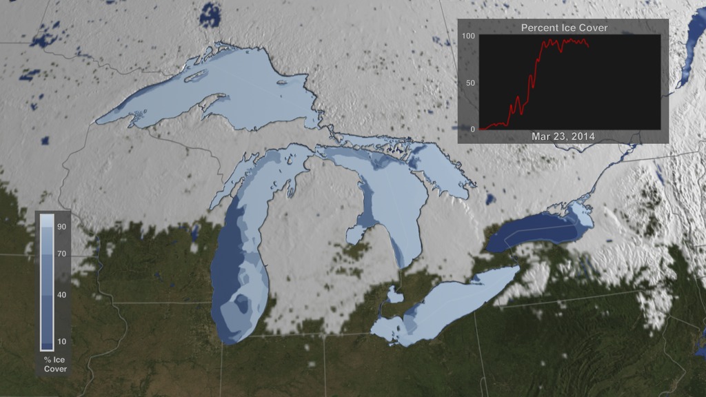
The Winter of 2013 – 2014: A Cold, Snowy and Icy Winter in North America
This animation shows the snow cover over North America during the 2013-2014 winter as well as the ice concentration over the Great Lakes. The date and a graph showing the percent of ice cover over the Great Lakes and Lake Superior is shown on this version. file size is 5.2 MB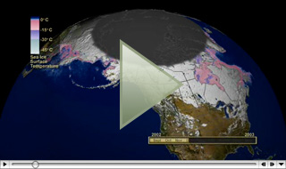
Snow Cover & Sea Ice Animation
This animation shows the advance and retreat of daily snow cover along with daily sea ice surface temperature globally from September 2002 through May 2003. file size is 31MB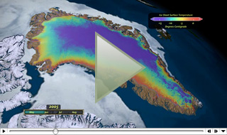
Surface Temperature of the Greenland Ice Sheet During the Summer of 2005
This animation shows daily surface temperature of the Greenland ice sheet from May 1 through September 1, 2005. An overlay contains a date bar, a color bar and text labels. file size is 14MB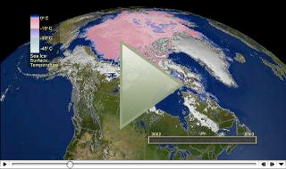
Daily Snow and Sea Ice Temperature over the North Pole
This animation shows the daily advance and retreat of snow cover, and sea ice surface temperature over the North Pole during the winter of 2002-2003. file size is 31MB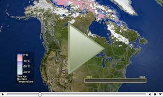
Daily Snow and Sea Ice Temperature over North America
This animation shows the daily advance and retreat of snow cover, and sea ice surface temperature over North America during the winter of 2002-2003. file size is 15MB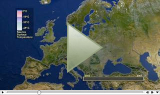
Daily Snow and Sea Ice Temperature over Europe
This animation shows the daily advance and retreat of snow cover, and sea ice surface temperature over Europe during the winter of 2002-2003. file size is 31MB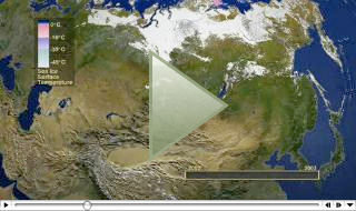
Daily Snow and Sea Ice Temperature over Asia
This animation shows the daily advance and retreat of snow cover, and sea ice surface temperature over Asia during the winter of 2002-2003. file size is 7MB
Intercomparison of Satellite-Derived Snow-Cover Maps
Dorothy K. Hall1, Andrew B. Tait2, James L. Foster1, Alfred T. C. Chang1, and Milan Allen3
1 Code 974, Hydrological Sciences, NASA/Goddard Space Flight Center, Greenbelt, MD 20771, dhall@glacier.gsfc.nasa.gov
2 Universities Space Research Association, NASA/Goddard Space Flight Center, Greenbelt, MD 20771.
3 National Operational Hydrologic Remote Sensing Center, Chanhassen, MN 55317.
ABSTRACT
In anticipation of the launch of the Earth Observing System (EOS) Terra, and the PM-1 spacecraft in 1999 and 2000, respectively, efforts are ongoing to determine errors of satellite-derived snow-cover maps. EOS Moderate Resolution Imaging Spectroradiometer (MODIS) and Advanced Microwave Scanning Radiometer-E (AMSR-E) snow-cover products will be produced. For this study we compare snow maps covering the same study area acquired from different sensors using different snow-mapping algorithms. Four locations are studied in: 1) Saskatchewan; 2) New England (New Hampshire, Vermont and Massachusetts) and eastern New York; 3) central Idaho and western Montana; and 4) North and South Dakota. Snow maps were produced using a prototype MODIS snow-mapping algorithm from Landsat Thematic Mapper (TM) scenes of each study area at 30-m and when the TM data were degraded to 1-km resolution. National Operational Hydrologic Remote Sensing Center (NOHRSC) 1-km resolution snow maps were also used, as were snow maps derived from ½° x ½° resolution Special Sensor Microwave Imager (SSM/I) data. A land-cover map derived from the International Geosphere-Biosphere Program (IGBP) land-cover map of North America was also registered to the scenes. The TM, NOHRSC and SSM/I snow maps, and land-cover maps were compared digitally. In most cases, TM-derived maps show less snow cover than the NOHRSC and SSM/I maps because areas of incomplete snow cover in forests (e.g., tree canopies, branches and trunks) are seen in the TM data, but not in the coarser-resolution maps. The snow maps generally agree with respect to the spatial variability of the snow cover. The 30-m resolution TM data provide the most accurate snow maps, and are thus used as the baseline for comparison with the other maps. Results show that the percent change in amount of snow cover, as compared to to the 30-m resolution TM maps, is lowest using the TM 1-km resolution maps, ranging from 0 to 40%. The highest percent change (>100%) is found in the New England study area, probably due to the presence of patchy snow cover. A scene with patchy snow cover is more difficult to map accurately than is a scene with a well-defined snowline such as is found on the North and South Dakota scene where the percent change ranged from 0 to 40%. There are also some important differences in the amount of snow mapped using the two different SSM/I algorithms because they utilize different channels.
Introduction
The launch of the Earth Observing System (EOS) Terra, and the PM-1 spacecraft in 1999 and 2000, respectively, will allow us to produce global snow maps, that are superior to those available today, from the EOS Moderate Resolution Imaging Spectroradiometer (MODIS) and the Advanced Microwave Scanning Radiometer-E (AMSR-E). Efforts are ongoing to determine errors of satellite-derived snow-cover maps, and these efforts will continue in the EOS era.
In previous work, we have estimated errors in snow maps in eight different land covers under conditions of continuous snow cover, using Landsat thematic mapper (TM) data and land-cover maps, and extrapolated those errors globally (Hall and others, 1998). For the present study, we compare snow maps derived from TM data, degraded to 1-km resolution, with National Operational Hydrologic Remote Sensing Center (NOHRSC) and Defense Meteorological Satellite Program (DMSP)/Special Sensor Microwave Imager (SSM/I) snow maps over four study areas located in North America (Table 1) to determine relative errors as compared to 30-m resolution TM-derived snow maps. The 30-m resolution TM snow maps were derived using the MODIS prototype algorithm, SNOWMAP (Hall and others, 1995; Klein and others, 1998a). These maps are considered to be the most accurate because of the good spatial resolution, and because some of the errors with this method of snow mapping have recently been evaluated under conditions of continuous snow cver (Hall and others, 1998). Two different algorithms were applied to the SSM/I data, and the results of a comparison of the resulting snow maps are also discussed. Results demonstrate some of the problems in quantitative comparison of snow maps derived from different sensors at different spatial resolutions. These problems will continue to plague researchers in the EOS era.
Background
EOS snow-cover products
The EOS Terra spacecraft will fly in a sun-synchronous, near-polar orbit with a 10:30 a.m. equatorial-crossing time and will include the MODIS instrument as part of its payload (Kaufman and others, 1998). The MODIS and AMSR-E instruments will be placed on the EOS first afternoon (EOS PM-1) spacecraft which is scheduled to be launched in 2000.
MODIS is a 36-channel spectroradiometer covering visible, near-, shortwave-infrared and infrared bands from 0.4-14 µm (Barnes and others, 1998). The AMSR-E is a twelve channel, six-frequency passive-microwave radiometer system. It measures brightness temperatures at 6.925, 10.65, 18.7, 23.8, 36.5, and 89.0 GHz in both vertical and horizontal polarizations.
MODIS-derived daily, global snow-cover maps are planned to be produced using data from the Terra and EOS PM-1 satellites, and both MODIS- and AMSR-E-derived snow maps will be produced from sensors on the PM-1 platform. Algorithms are being developed that will use both AMSR-E and MODIS data, together, to map global snow cover (Tait and others, 1999 and in press).
A fully-automated algorithm, SNOWMAP, has been developed that will map global snow cover, cloud-cover permitting, on a daily basis at 500-m spatial resolution using MODIS data (Hall and others, 1995; Riggs and others, 1996; Klein and others, 1998a). Shortly after launch, there will be daily and 8-day composite global snow-cover products at 500-m resolution, and daily and 8-day and monthly-composite climate-modeling grid (CMG) products at 1/4° X 1/4° spatial resolution. MODIS snow and ice data products will be archived at and distributed by the National Snow and Ice Data Center (NSIDC) in Boulder, Colorado (Scharfen and others, 1997).
Detailed studies of the SNOWMAP algorithm have been conducted in many different land covers, resulting in estimates of snow-mapping errors in at least eight individual land-cover classes under conditions of continuous snow cover (Hall and others, 1998). Preliminary results, under cloud-free conditions, show the highest average errors in forested areas (15%) and the lowest average errors in non-forested areas (5%). Errors are expected to be greater when snow cover is not continuous, and are expected to be greatest in alpine areas containing patchy snow cover (J. C. Shi/UCSB, written communication, 1999).
Currently, a global, daily snow-cover data set at 500-m resolution (or better) does not exist, therefore, a direct comparison of the MODIS and AMSR-E-derived products with "actual" global snow cover will not be possible following the launches of Terra and PM-1. Instead, the EOS snow maps will be compared with other hemispheric-scale maps such as the Northern Hemisphere weekly snow-cover maps produced by the National Oceanic and Atmospheric Administration (NOAA) National Environmental Satellite, Data and Information Service (NESDIS), and maps prepared by NOHRSC. Precise errors of these snow maps have not been established. The EOS snow maps will also be compared with maps derived from passive-microwave data (e.g., Chang and others, 1987 and 1997; Grody and Basist, 1996; Tait and others, in press) from the SSM/I. At regional and local scales, MODIS snow-cover maps will be validated using snow-cover maps derived from the Landsat-7 Enhanced Thematic Mapper Plus (ETM+), launched on 15 April 1999, and Terra's Advanced Spaceborne Thermal Emission and Reflection Radiometer (ASTER).
NOHRSC snow maps
The Geostationary Operational Environmental Satellite (GOES) imager scans parts of the Earth every fifteen minutes. The visible images are navigated and registered using 169 landmarks in the northern and southern hemispheres. The navigation specifications require the visible data to be within 4 km and infrared data to be within 6 km. Using 15 minute visible imagery during the past 52 weeks, 90 percent or greater of landmarks met specifications for the north-south direction (except for three weeks) and 95 percent or greater of landmarks met specifications for the East-West direction (except for two weeks).
Once daily, from Saturday through Thursday GOES East and GOES West infrared (bands 2, 4, and 5) and water vapor (band 3) images are resampled to match the 1-km resolution of the visible data using an inverse distance function. Each pixel in the visible band is normalized to solar noon using a simple cosine correction. The normalized visible image and the reprojected and resampled infrared bands are used as input to an algorithm that produces 32-bit images of cloud and snow/cloud. Each image is given an 80-byte header, which contains the ancillary information required to read and utilize the images. The three images are divided into smaller, more manageable images for analysis. Each subdivided image is analyzed to produce a cloud mask image and a snow/cloud image. A coastline vector file is layered on one of the visible images to derive the north-south and east-west shift required to align or register the final snow-cover image. The cloud and snow/cloud images are merged to produce an image of snow, cloud, and no-snow/no-cloud for each subdivided image; the smaller images are mosaicked to produce an unregistered east or west snow-cover map. Alphanumeric tabulations of percent of snow cover by hydrologic basin and elevation zone are produced and are made available on the NOHRSC web site (http://www.nohrsc.nws.gov/), and are sent to the National Weather Service (NWS) offices over the NWS communications lines and sent by ftp over the Internet to interested agencies.
Land-cover maps
To determine land-cover type, International Geosphere-Biosphere Project (IGBP) land-cover maps of North America developed from 1-km Advanced Very High Resolution Radiometer (AVHRR) data are used (Loveland and Belward, 1997). These maps are based on monthly normalized difference vegetation index (NDVI) composites from 1992 and 1993. Using these maps, Hall and others (1998) classified the Northern Hemisphere into the following eight land-cover classes: forest, mixed agriculture and forest, barren/sparsely vegetated, tundra, grasslands/shrublands, wetlands, permanent snow and ice, and water, and estimated snow-cover mapping errors in each land-cover class for continuous snow-cover conditions based largely on field studies.
Study Areas and Satellite Data
TM, NOHRSC and SSM/I data were acquired for four study areas located in Canada and the United States: 1) Saskatchewan, Canada, 2) New England (Massachusetts, New Hampshire and Vermont) and eastern New York, 3) central Idaho and western Montana, and, 4) parts of North and South Dakota in the United States (Table 1). The site in Saskatchewan is characterized by gentle relief and rolling hills (interior lowlands) and is composed predominately of boreal forest (aspen and spruce), and some mixed agriculture and forest. It is located in an area of prairie snow cover according to Sturm and others (1995). Land cover in the New England study area is predominately composed of northern hardwood forests, and the snow cover is maritime snow cover (Sturm and others, 1995). In the Idaho study area, terrain is mountainous (northern Rocky Mountains) and forested (mainly fir trees), and the snow cover is prairie, alpine or maritime (Sturm and others, 1995). In the study area in North and South Dakota, the terrain is mainly flat (the Great Plains), and land cover is composed of grassland/shrubland in the west and mixed agriculture and forest in the east, and the snow cover is classified by Sturm and others (1995) as prairie snow.
The SNOWMAP algorithm was applied to the 30-m and 1-km resolution TM data (Klein and others, 1998a) to map snow. Using the SSM/I data, two different algorithms were used to map snow. The Grody and Basist (1996) method uses the difference between the microwave brightness temperature (TB) at 37 and 19 GHz, and at 85 and 22 GHz vertical polarizations, and a decision tree whereby filters are used to isolate the snow-cover signature. The Chang and others (1997) method (without forest-cover corrections) was also used. This is based on the difference between the 19 and 37 GHz channels,
where SD is snow depth (in cm).
One of the main problems with SSM/I-derived snow-cover maps is the presence of melting snow. Liquid water coating snow grains absorbs microwave radiation producing an increase in TB. To minimize this problem, only the early-morning satellite observations were used because this is when the surface temperature is generally the coldest.
The SSM/I maps may not cover the exact same areas on the ground as do the TM and NOHRSC maps, although efforts were made to register the data. It is possible that the SSM/I maps are as much as 25 km offset from the other maps. The lack of ground-control points observable on the SSM/I data meant that the registration could only be done using latitude and longitude lines.
The spatial resolutions of the various snow maps discussed herein are different. TM maps have 30-m resolution and are also degraded to 1-km resolution, while the NOHRSC maps have 30 arc-second resolution (approximately 1-km resolution at the equator). The resolution of the SSM/I snow maps is 1/2° X 1/2°; at a latitude of 50°, this is approximately 35 X 55 km.
Results and Discussion
The NOHRSC and SSM/I maps were registered digitally to the Landsat TM-derived maps. The latitude and longitude of the center of each SSM/I pixel were known. Also, we knew the corner latitude and longitude of each TM scene. To obtain the best possible co-registration, we chose sections of the SSM/I data that matched the latitude and longitude boundaries of the TM scenes most closely. A condition to these selections was that the SSM/I "box" was slightly larger than the TM scene, so that the TM scene could fit inside the SSM/I box. We were then able to extract the SSM/I data according to the corner latitudes and longitudes of the TM scene. If we were to shift the SSM/I box up/down or left/right we would only be getting farther from the optimum co-registration.
Since all of the maps were registered (i.e., the SSMI and NOHRSC maps were registed to the TM-derived maps), the percentage of snow cover was easily determined from the TM, NOHRSC and each of the SSM/I maps for the area covered by TM data (Table 2).
The 30-m resolution TM data were degraded to 1-km resolution in the following way. Each band of the TM data that is used in the SNOWMAP algorithm was reprojected from 30- to 25-m spatial resolution separately. Then 40 X 40 pixels were averaged to equal the spatial area (1600 pixels X 625 m2) of a 1-km pixel (100,000 m2). The data from individual bands, at 1-km resolution, were then used in the MODIS prototype algorithm to create a snow-cover map. The SNOWMAP algorithm was applied to the data after the degradation in spatial resolution.
Saskatchewan
The 27 January 1996 30-m resolution TM snow map (TM-1) of southern Saskatchewan showed 70% snow cover (Figure 1). The boreal forest in the northern part of the scene contains both coniferous and deciduous trees. Unless there has been a recent snowfall, the tree canopies, branches, stems and trunks will likely be mapped as non-snow covered because the snow is often blown or falls from a tree canopy, or the snow sublimates over time. Previous work has shown that it is very difficult to map snow through both dense coniferous and dense deciduous forests (Hallikainen and others, 1988; Foster and others, 1994; Hall and others, 1998). While some areas in the central and western parts of the TM scene are not mapped as snow covered, the southern part of the scene which is composed of mixed agricultural and forest (but is predominately agricultural land), is nearly 100% snow covered as seen on the TM-derived maps. The snow map created from the TM data, degraded to 1-km resolution (TM-2), shows 86% snow cover. The NOHRSC and both SSM/I-derived snow maps all show 100% snow cover for the scene (Table 2).
New England
Most (96%) of the area included in the 21 January 1997 TM scene of New England (including eastern New York, parts of Vermont, New Hampshire and Massachusetts) is composed of forest (Figure 2).While the TM 30-m resolution map shows only 37% snow cover, the TM 1-km map shows 52%, and the NOHRSC and SSM/I-1 maps, show 77% and 73% snow cover, respectively (Table 2). Across most of the scene, snow cover was intermittent as determined from field work and meteorological-station data (Bayr and others, 1997; NOAA, 1997a; Klein and others, 1998b; Tait and others, 1999). (Note that the NOAA meteorological stations tend to be in open areas where less snow may be present than in the forests.) For example, Berlin, New York had about 13 cm and Glens Falls, New York had 10 cm (NOAA, 1997a). In Keene, New Hampshire, NOAA data show 5 cm of snow on the ground on 21 January 1997, though reports from Keene indicate patchy snow cover in the surrounding areas on that date (Klaus Bayr, written communication, 1999). To the east, in Manhester, New Hampshire, there was no snow reported on the ground (NOAA, 1997b). In the southeastern part of the scene, in Massachusetts, the TM, NOHRSC (Figure 2 and Figure 3) and the SSM/I-derived maps are shown as snow-free. This is consistent with the meteorological-station data of that area, for example, New Salem, Massachusetts, had only a trace of snow on the ground on 21 January (NOAA, 1997a).
The SSM/I-derived snow map using the Chang and others (1997) algorithm, (SSM/I-2), without forest-cover correction, shows 96% of the New England scene as being snow free. This is probably due to the fact that the snow is shallow and wet and therefore its signature is similar to the surrounding snow-free ground. Also, this is a forested area which often causes problems for snow mapping using SSM/I data since emission from trees increases the TB (Foster and others, 1994) especially under patchy-snow conditions. The SSM/I-1 algorithm utilizes the 85-GHz channel which is more sensitive to snow cover, and therefore maps shallower snow than does the SSM/I-2 algorithm. This may be why the SSM/I-1 algorithm maps more snow cover in this scene than does the SSM/I-2 algorithm.
The New England snow maps (with the exception of the SSM/I-2 map) generally agree with respect to the location of snow cover, but not with respect to amount of snow cover. Probably the main reason that the TM map shows less snow cover than the other maps (Table 2) is that the intermittent snow in the forests in the area is mapped as full snow cover on the NOHRSC and SSM/I-1 maps, and, more correctly, as partial snow cover on the TM map.
In the forested New England study area, there is patchy snow cover in New Hampshire, Vermont and New York, but in Massachusetts (southeastern part of the scene) the area is basically snow free according to meteorological-station data. All of the snow maps show this area to be snow free.
Idaho
In Idaho, on the 28 January 1998 TM-1 snow map, in a predominately forested site, snow is mapped over 62% of the scene while the TM-2, NOHRSC and both SSM/I maps show greater amounts of snow cover (Table 2). The TM-1 map does not show continuous snow cover in the forests, while the other snow maps do (Figure 4 and Figure 5). Mountain shadows are present and are incorrectly mapped as being snow free using the TM-1 and -2 maps. The apparently snow-free area on the TM maps is cloudcover (see arrow on Figure 4).
On the Idaho maps, a non-snow-covered area is shown in the southwestern part of the scene on both TM and the NOHRSC maps (Figure 4), and the SSM/I-1 map (Figure 5). The nearby station at Emmett, Idaho, just south of the scene, reported no snow cover (NOAA, 1998a). Farther to the west, the TM and both of the SSM/I maps show continuous snow cover. Meteorological-station data are sparse to the east of Emmett, but point values show 25-71 cm of snow on the ground in this area. For example, there were 51 cm in Idaho City, Idaho (NOAA, 1998a) in an area that is shown as snow free on the NOHRSC snow maps.
Other problems are evident. Both SSM/I maps show a well-delineated snowline in the western part of the scene where there is no snowline according to the TM and NOHRSC data. If the snow cover is patchy and thin, the large SSM/I pixels may not detect enough of a signal change to map the whole pixel as snow, and thus both SSM/I algorithms map the western part of the scene as snow-free.
In Idaho, a mountainous area, continuous snow cover is not mapped in mountain shadows using the TM data, but is mapped using the coarser-resolution data. In this case, it is believed that the TM-1 snow map underestimates the amount of snow cover that is present.
North and South Dakota
In North and South Dakota, a snowline is visible on all of the 7 and 8 February 1998 snow maps (Figure 6 and Figure 7). The eastern part of all of the maps is generally snow covered, while the southern and southwestern parts are snow free. The snowline, as seen on the TM-derived maps, follows closely the boundary between the grassland/shrubland land-cover class to the west (which is snow free) and the mixed vegetation and forest class (which is snow covered) to the east (Figure 6). The snow cover remains longer in the forest than it does in the grassland/shrubland, and this is the reason that there is such an obvious snowline on the TM-derived snow maps. This appears to be an accurate depiction of the snow-cover situation, and is corroborated by the NOAA meteorological-station data showing, for example, no snow cover in Pollock, South Dakota (NOAA, 1998b), west of the snowline, and 13 cm in Jamestown, 20 cm in Cooperstown and 10 cm of snow cover in Edgely, North Dakota on 7 February 1998 (NOAA, 1998c), east f the snowline. The NOHRSC map also shows a well-defined snowline, but in a slightly different place than shown on the TM-derived maps. In this case, it was difficult to register the TM and NOHRSC data, due to a lack of ground-control features, and therefore the positions of the snowlines may not match due to mis-registration.
Both SSM/I-derived snow maps show a well-defined snowline in the southwestern part of the scene. In addition, the SSMI-1 map shows a snow-free area in the eastern part of the scene in a location that is snow covered according to the other maps and the meteorological-station data. These snow-free pixels are the result of the algorithm's precipitation filter which indicates that it may have been raining or snowing at the time the data were acquired. Standley and Barrett (1999) have used the infrared data from the DMSP Operational Line Scanner (OLS), in combination with the SSM/I data to map snow more accurately than when using the SSM/I data alone. This is because the infrared temperature of snow cover is generally greater than that of the precipitating clouds.
There was very little change in the amount of snow on the TM-1 and -2 maps (64%) in the North and South Dakota study area. Though the TM-2 map showed slightly more snow cover than did the TM-1 map, as a percentage of the total area of the scene, both rounded off to 64%. The NOHRSC 1-km resolution maps show less snow (57%), while the SSM/I-1 and -2 maps show 89 and 86% snow cover, respectively. In terms of spatial coverage, this area provided more consistent results among the snow maps than did the maps with patchy snow cover, probably because it is much easier to map continuous snow cover with a well-defined snowline accurately than to map patchy snow cover accurately.
Discussion
Because of the good (30 m) spatial resolution of the TM sensor, and the fact that the SNOWMAP algorithm has been evaluated for accuracy in different land covers, the assumption is that, of the snow maps studied in this paper, the 30-m resolution Landsat TM-derived snow maps (TM-1) are the most accurate. The snow maps derived from TM data (1-km resolution), NOHRSC maps and both SSM/I maps were compared to the TM (30-m resolution) maps. Percent change in snow cover mapped, relative to the TM 30-m resolution data is shown in Figure 8. This, however, just addresses the accuracy in terms of the total amount of snow mapped, and not the accuracy in terms of the location of the snow cover, and for this reason may be misleading. Furthermore, it is expected that the TM-2 maps should be the most similar of all the maps, to the TM-1 maps because the same algorithm was used to calculate snow cover using both the 30-m and 1-km resolution TM maps. The NOHRSC maps are generally accurate depictions of the location of sow cover, but show more snow cover than is probably present because the tree canopy, branches and stems are actually not snow covered as seen on the TM data. When the TM data are degraded to 1-km spatial resolution, more snow is generally mapped.
The important role of land cover in snow-cover distribution is seen in the North and South Dakota scene where there is a distinct snowline at a clear demarcation between the grassland/shrubland and the mixed agriculture and forest land-cover classes (Figure 6). This snowline is apparent on all of the satellite-derived maps.
The SSM/I maps are considered to be the least accurate in terms of mapping the location of snow cover accurately primarily because of the coarse resolution of the data. There is confusion in the SSM/I-2 maps in patchy snow in forests in the New England study area. The SSM/I-1 algorithm maps precipitation as non-snow cover and maps more snow cover in the eastern part of the North and South Dakota scene than is present. In Saskatchewan, the SSM/I maps both show 100% snow cover. Due to the coarse resolution, the signature of the snow-free tree canopies and trunks is not detected because the algorithms cannot delineate sub-grid-size features. Even in continuous snow cover, snow-free areas exist and should be mapped as being snow free if the resolution of a satellite sensor is good enough.
Conclusions
This study demonstrates some of the difficulties involved in intercomparing satellite-derived snow-cover maps. First, we do not know which map is the most accurate though we make the assumption, in this work, that the highest-resolution map (30-m resolution map derived from TM data) is the most accurate. In addition, since different satellite sensors are used to derive the maps, different algorithms are used. Furthermore, the maps are at different spatial resolutions, thus further complicating the comparisons. More such intercomparisons will be accomplished following the launch of the MODIS sensor on the Terra spacecraft. It will be possible to use Landsat-7 data to derive snow-cover maps and compare those with MODIS, SSM/I and AMSR-E maps. As the EOS MODIS and AMSR-E data sets become available, and such studies are repeated, we will be able to reduce the uncertainties in the accuracy assessments of various snow maps.
Acknowledgments
The authors would like to thank Janet Chien of General Sciences Corporation (GSC), Laurel, MD for image processing, and Meg Larko of GSC for obtaining the SSM/I data, and Andrew Klein of Texas A & M University, College Station, TX, Alex Moore of Hartwick College, Oneonta, NY and Klaus Bayr of Keene State College, Keene, NH, for obtaining field measurements in the New England/New York study area during February 1997.
References
Bayr, K.J., J.C. Goumas and K.A. Picard, 1997: Description of snow measurements - February 9, 1997 - Keene, New Hampshire area: Tenant Swamp, Spoffort Lake, Bretwood Golf Course, Keene State College, Keene, NH.
Barnes, W.L., T.S. Pagano and V.V. Salomonson, 1998: Prelaunch characteristics of the Moderate Resolution Imaging Spectroradiometer, IEEE Transactions on Geoscience and Remote Sensing, 36(4):1088-1100, 1998.
Carroll, T.R., 1990: Operational airborne and satellite snow cover products of the National Operational Hydrologic Remote Sensing Center, Proceedings of the forty-seventh annual Eastern Snow Conference, June 7-8, 1990, Bangor, Maine, CRREL Special Report 90-44, 1990.
Chang, A.T.C., J.L. Foster and D.K. Hall, 1987: Nimbus-7 derived global snow cover parameters, Annals of Glaciology, 9:39-44, 1987.
Chang, A.T.C., J.L. Foster, D.K. Hall, B.E. Goodison, A.E. Walker, J.R. Metcalfe and A. Harby, 1997: Snow parameters derived from microwave measurements during the BOREAS winter field campaign, Journal of Geophysical Research, 102(D4):29,663-29,671.
Foster, J.L., A.T.C. Chang and D.K. Hall, 1994: Snow mass in boreal forests derived from a modified passive microwave algorithm, Multispectral and Microwave Sensing of Forestry, Hydrology, and Natural Resources, E. Mougin, K.J. Ranson and J.A. Smith (ed.), 26-30 September 1994, Rome, Italy, pp. 605-617.
Grody, N.C. and Basist, A.N., 1996: Global identification of snowcover using SSM/I measurements, IEEE Transactions on Geoscience and Remote Sensing, 34(1):237-249.
Hall, D.K., G.A. Riggs and V.V. Salomonson, 1995: Development of methods for mapping global snow cover using Moderate Resolution Imaging Spectroradiometer (MODIS) data, Remote Sensing of Environment, 54:127-140.
Hall, D.K., J.L. Foster, V.V. Salomonson, A.G. Klein and J.Y.L. Chien, 1998: Error analysis for global snow-cover mapping using satellite data in the Earth Observing System (EOS) era, Proceedings of IGARSS'98, pp. 1524-1526.
Hallikainen, M., T., P. A. Jolma, and J.M. Hyyppa, 1988: Satellite microwave radiometry of forest and surface types in Finland, IEEE Transactions on Geoscience and Remote Sensing, 26:622-628.
Kaufman, Y.J., D.D. Herring, K.J. Ranson and G.J. Collatz, Earth observing system AM1 mission to Earth, 1998: IEEE Transactions on Geoscience and Remote Sensing, 36(4):1045-1055.
Klein, A.G., D.K. Hall and G.A. Riggs, 1998a: Improving snow-cover mapping in forests through the use of a canopy reflectance model, Hydrological Processes, 12(10-11):1723-1744.
Klein, A.G., D.K. Hall and K. Seidel, 1998b: Algorithm intercomparison for accuracy assessment of the MODIS snow-mapping algorithm, Proceedings of the 55th Eastern Snow Conference, 2-3 June 1998, Jackson, NH, pp.37-45.
Loveland, T.R., and A.S. Belward, 1997: The IGBP-DIS global 1 km land cover data set, DESCover: first results, International Journal of Remote Sensing, 18(15):3289-3295.
NOAA, 1997a: Climatological Data of New England, Asheville, NC.
NOAA, 1997b: Climatological Data of New York, Asheville, NC.
NOAA, 1998a: Climatological Data of Idaho, Asheville, NC.
NOAA, 1998b: Climatological Data of South Dakota, Asheville, NC.
NOAA, 1998c: Climatological Data of North Dakota, Asheville, NC.
Riggs, G.A., D.K. Hall and V.V. Salomonson, 1995: Recent progress in development of the Moderate Resolution Imaging Spectroradiometer snow cover algorithm and product, Proceedings of IGARSS'96, Lincoln, NE, pp.139-141, 1996.
Scharfen, G.R., D.K. Hall and G.A. Riggs, 1997: MODIS snow and ice products from the NSIDC DAAC, Proceedings of SPIE, 27 July - 1 August 1997, San Diego, CA, pp. 143-147, 1997.
Standley, A.P. and E.C. Barrett, 1999: The use of coincident DMSP SSM/I and OLS satellite data to improve snow cover detection and discrimination, International Journal of Remote Sensing, 20(2):285-305.
Sturm, M., J. Holmgren and G.E. Liston, 1995: A seasonal snow cover classification system for local to regional applications, Journal of Climate, 8(5):1261-1283.
Tait, A.B., D.K. Hall, J. Foster, A. Chang and A. Klein, 1999: Detection of snow cover using millimeter-wave imaging radiometer (MIR) data, Remote Sensing of Environment, 68:53-60.
Tait, A.B., D.K. Hall, J.L. Foster and A.T.C. Chang, in press: High frequency passive microwave radiometry over a snow covered surface in Alaska, Photogrammetric Engineering and Remote Sensing.
List of Tables
Table 1. Satellite data used in this study.