
More Information
view allVideos
Videos
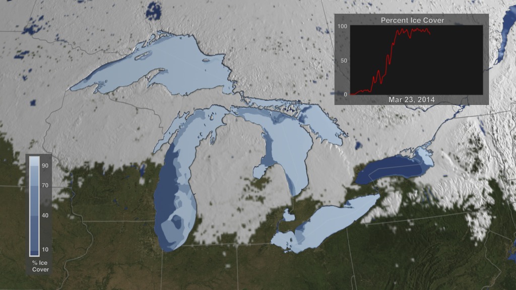
The Winter of 2013 – 2014: A Cold, Snowy and Icy Winter in North America
This animation shows the snow cover over North America during the 2013-2014 winter as well as the ice concentration over the Great Lakes. The date and a graph showing the percent of ice cover over the Great Lakes and Lake Superior is shown on this version. file size is 5.2 MB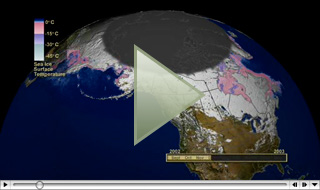
Snow Cover & Sea Ice Animation
This animation shows the advance and retreat of daily snow cover along with daily sea ice surface temperature globally from September 2002 through May 2003. file size is 31MB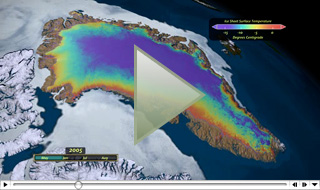
Surface Temperature of the Greenland Ice Sheet During the Summer of 2005
This animation shows daily surface temperature of the Greenland ice sheet from May 1 through September 1, 2005. An overlay contains a date bar, a color bar and text labels. file size is 14MB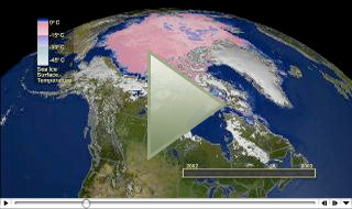
Daily Snow and Sea Ice Temperature over the North Pole
This animation shows the daily advance and retreat of snow cover, and sea ice surface temperature over the North Pole during the winter of 2002-2003. file size is 31MB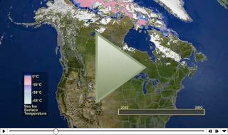
Daily Snow and Sea Ice Temperature over North America
This animation shows the daily advance and retreat of snow cover, and sea ice surface temperature over North America during the winter of 2002-2003. file size is 15MB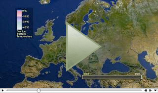
Daily Snow and Sea Ice Temperature over Europe
This animation shows the daily advance and retreat of snow cover, and sea ice surface temperature over Europe during the winter of 2002-2003. file size is 31MB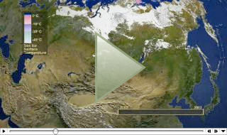
Daily Snow and Sea Ice Temperature over Asia
This animation shows the daily advance and retreat of snow cover, and sea ice surface temperature over Asia during the winter of 2002-2003. file size is 7MB
Sea Ice Extent and Classification Mapping with the Moderate Resolution Imaging Spectroradiometer Airborne Simulator
George A. Riggs1, Dorothy K. Hall2, and Steven A. Ackerman3
1 Research and Data Systems Corp. 7833 Walker Drive, Suite 550, Greenbelt, MD, 20770.2 Code 974, NASA Goddard Space Flight Center, Greenbelt, MD, 20771.
3 Cooperative Institute for Meteorological Satellite Studies, University of Wisconsin-Madison, Space Science and Engineering Center, 1225 West Dayton Street, Madison, WI 53706.
ABSTRACT
An algorithm for mapping sea ice extent and generalized classification of sea ice by reflective and temperature characteristics with Moderate Resolution Imaging Spectroradiometer (MODIS) Airborne Simulator (MAS) data is presented. The algorithm was tested using a MAS scene over the Bering Sea near St. Lawrence Island, Alaska, USA, acquired 8 April 1995. Clouds were masked with the University of Wisconsin cloud masking algorithm. Ice surface temperature was estimated with a split-window technique. Sea ice extent and generalized type of sea ice were identified based on reflective characteristics and estimated ice surface temperature using a grouped criteria technique. Resulting maps were consistent with visual interpretation and with sea ice extent and type information reported in prior studies of the region. Published by Elsevier Science Inc.
Introduction
At its seasonal maximum, sea ice covers roughly 10% of the Earth's oceans (Carsey, et al., 1992). It varies greatly in both extent and thickness due to the combined effect of dynamic and thermodynamic processes. In the Arctic it varies from a March maximum of approximately 15 x 106 km2, to a September minimum of about 8 x 10⁶ km2 (Parkinson and Gloersen, 1993). In the Antarctic, a maximum extent of approximately 20 x 106 km2 occurs in September while a minimum of 4 x 10⁶ km2 occurs in February (Parkinson and Gloersen, 1993). The presence of sea ice influences atmospheric and oceanic temperature and circulation patterns, and reduces the amount of solar radiation absorbed in the ocean. Sea ice and its associated snow cover serves as a strong insulator, restricting exchanges of heat, mass, momentum and chemical constituents between the atmosphere and the ocean. With an ice cover, only 30-50% of the incident solar radiation is absorbed. Without sea ice, 85-95% of the incident solar radiation is absorbed by the oceans (Washington and Parkinson, 1986).
Satellite remote sensing is an important tool for global mapping of sea ice extent, concentration, type and temperature. Two classes of sensors, microwave and multi-spectral radiometers, are typically used. The ability of microwave instruments, e.g. the special sensor microwave imager (SSM/I) and synthetic aperture radars (SARs), to collect data through cloud cover and polar darkness makes them well suited for monitoring of sea ice extent and concentration. Passive-microwave sensors acquire data at spatial resolutions of 25-50 km, while SARs may acquire data at 25 m resolution. However, microwave instruments cannot collect data on spectral reflectance or surface temperature which is needed for analysis of energy exchange between the ocean and atmosphere. Thus, multispectral radiometers also play an important role in sea ice research.
Multi-spectral radiometers, e.g., the Advanced Very High Resolution Radiometer (AVHRR), the Moderate Resolution Imaging Spectroradiometer (MODIS) and the MODIS Airborne Simulator (MAS) can be used for determination of sea ice extent, temperature, albedo, movement, type, and concentration at resolutions of 250 m - 1 km. After its launch in 1999 on the Earth Observing System (EOS) AM-1 platform, MODIS will provide, data from 36 spectral bands from visible to thermal infrared (0.45 to 14.4 µ m)
at a spatial resolution of 250 - 1000 m. However, cloud cover and polar darkness preclude continuous spatial and temporal coverage with those sensors.
The prototype of the MODIS sea ice algorithm is described in this paper, which used MAS to develop the sea ice mapping methodology. The algorithm will generate maps of sea ice extent as determined by reflectance characteristics and estimated ice surface temperature (IST) and will include the estimated IST as part of the data product. The product will be produced globally at 1 km spatial resolution. In the EOS era, MODIS will be used to generate a standard data product in the Earth Observation System Data Information System (EOSDIS).
Data Description
MODIS Airborne Simulator
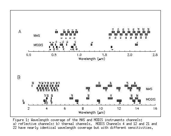
The MAS is a multi-spectral imaging spectrometer that measures reflected solar and emitted thermal radiation between 0.55 and 14.2 µ m in 50 narrow-band channels, that is flown aboard a NASA ER-2 aircraft. Nineteen of the 50 channels of the MAS have comparable channels on the MODIS (Figures 1a and 1b). MODIS channels 8-16, designed for ocean color applications, are shown in Figures 1a and 1b for completeness but may be of limited use over sea ice due to potential sensor saturation. At a nominal aircraft altitude of 20 km, MAS provides imagery with a swath width of 37 km and a pixel spatial resolution of 50 m at nadir. The MAS was built to support development of MODIS remote-sensing algorithms. A detailed description of the MAS, some MAS applications and field campaigns can be found in King et al. (1996) or at the MAS World Wide Web site (URLs are listed under the Relevant World Wide Web sites heading). A description of the MODIS instrument can be found in Barnes et al. (1998) or at the MODIS World Wide Web site.
Test Scene
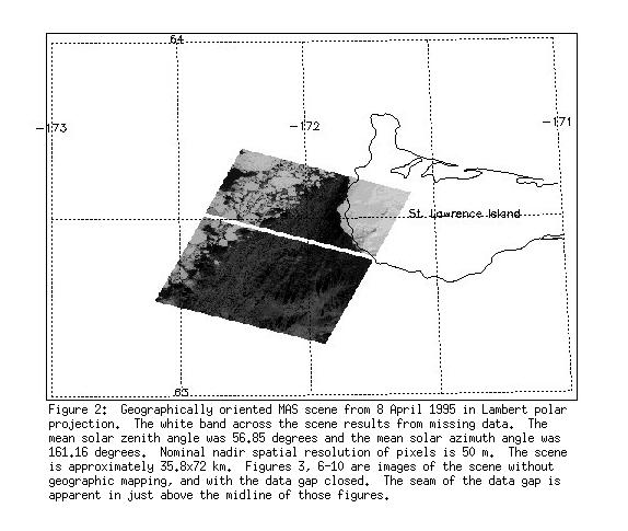
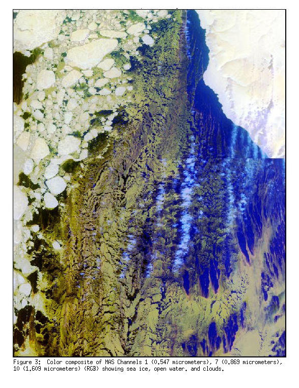
A MAS scene acquired on 8 April 1995 during the Alaska-April95 aircraft campaign was selected for its good combination of sea ice types, open water and clouds. The scene is located in the Bering Sea with a segment of the southwest coast of St. Lawrence Island included (Figure 2) and has a center location of approximately 63.42° north latitude, 172.10° west longitude. The flight direction is oriented northeast to southwest. A three channel (MAS channels 1,7,10) color composite of the scene is shown in Figure 3 and is used as a reference image on which algorithm results are overlaid.
Sea Ice Algorithm
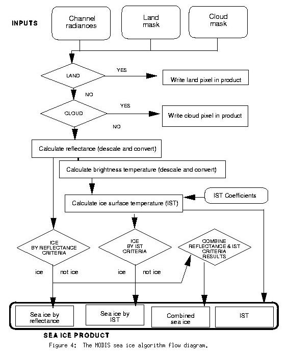
The primary purpose of the MODIS sea ice algorithm is to map sea ice extent. A potential secondary purpose is the creation of thematic maps showing generalized sea ice classes. The algorithm identifies sea ice by reflective characteristics and ice surface temperature, generating a four part data product. A grouped criteria methodology is employed to identify sea ice on a per pixel basis. The rationale for using the grouped criteria methodology is that the criteria are robust, can be easily modified or changed and can be dynamically linked with geographic or seasonal parameters affecting identification of sea ice, and is amenable to enhancements derived from future studies and independent validation. A flow diagram of the algorithm is depicted in Figure 4. The University of Wisconsin cloud mask (UWCM) algorithm was chosen to mask clouds because it will produce the standard MODIS cloud mask data product. The UWCM algorithm uses select channels in the visible, infrared and thermal channels in various cloud detection tests (single band thresholds, ratios, channel differences and others) with threshold rules for detection of cloud. Experience gained with the UWCM using the MAS is directly applicable to cloud masking with MODIS. A brief background discussion of sea ice reflectance characteristics and ice surface temperature calculation is presented, followed by descriptions of groups of criteria applied in the algorithm.
Sea Ice Reflective Characteristics
Observations of sea ice reflectance reported in the literature commonly cover the 0.4 - 1.0 µ m range (e.g. Perovich, 1990; De Abreu et al., 1995) and sometimes extend out to approximately 2.4 µ m (e.g. Grenfell and Perovich 1984; Perovich et al., 1986). Snow-covered, opaque, white sea ice, thick first-year ice and multiyear ice typically exhibit maximum reflectance between 0.4 - 0.8 µ m,
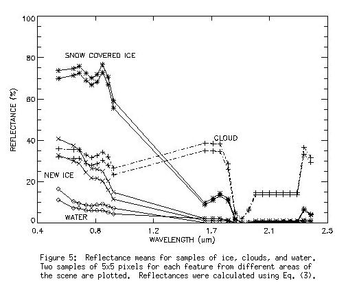
decreasing into the near-infrared, reaching a reflectance minimum at approximately 1.6 µ m, then rising again to a peak at approximately 1.9 µ m. Field observations show that sea ice is predominately snow-covered (Schlosser, 1988) and that this snow is usually present within a few days of formation (Perovich, 1990). Young sea ice (e.g., grease ice, nilas, young gray) has lower spectral albedos (in the range of 0.10 - 0.40) than older sea ice over the 0.4 - 0.8 µ m region. At longer wavelengths (› 1.0 µ m) the spectral albedo of young sea ice decreases to a value similar to older sea ice (Schlosser, 1988; Perovich, 1990; Allison et al., 1993). Sea ice undergoing ablation and containing melt ponds has decreasing reflectance from 0.6 to 0.8 µ m, followed by steady uniform low reflectance to approximately 1.6 µ m (Grenfell and Perovich, 1984; De Abreu et al., 1995). Reflectance curves (Figure 5) constructed from the mean reflectance of each MAS band from two spatially separated 5 x 5 pixel samples band of ice, cloud and water in the scene show reflectance features consistent with those reported in the sea ice observation studies discussed above. Using these sample curves from the scene and above studies as background, the sea ice reflectance criteria were developed to identify snow-covered sea ice and new sea ice.
Ice Surface Temperature
Split-window techniques are employed to determine sea-surface temperature (e.g. McMillin and Crosby, 1984; Minnett, 1990) or ice-surface temperature (e.g. Key and Haefliger 1992; Massom and Comiso, 1994; Yu et al., 1995; Key et al., 1997). Split-window techniques allow for correction of atmospheric effects, primarily water vapor, and yield reasonably accurate sea surface temperature (SST) or ice surface temperature (IST) estimates.
Instrument channels used for estimation of surface temperature with the split-window technique are centered at approximately 11.0 and 12.0 µ m. Several investigators (e.g. Key and Haefliger, 1992; Lindsay and Rothrock, 1993; Massom and Comiso, 1994; Yu et al., 1995; Key et al., 1997) have employed variations of the split-window technique for estimation of IST in polar regions using the AVHRR and other instruments. In most studies, accuracy of the split-window technique has been enhanced by adding predictor variables to account for effects such as sensor scan angle. Accuracy of the estimate of IST may be increased by regression of the estimated IST with temperatures modeled from radiative transfer models or with observed surface temperatures (e.g. Minnett, 1990; Key and Haefliger, 1992; Lindsay and Rothrock, 1993; Key et al., 1997). IST accuracy of 0.5 - 1.5 K relative to measured or modeled surface temperatures has been reported by investigators using the split-window technique.
The technique of Key et al. (1997) was adapted for estimating IST using MAS data. MAS channels 45 and 46, centered approximately at 11.0 and 12.0 µ m, respectively (Figure 1b), are used to determine IST. IST for MAS data is estimated using the equation
IST = a + bT45 + c(T45 - T46) + d[(T45 - T46) * sec(theta - 1)], (1)
where
IST -- ice surface temperature (K)
a,b,c,d -- are coefficients determined from multilinear regression of brightness temperatures to estimated surface temperatures (4)
T45 -- brightness temperature of MAS channel 45 (11.0 m m)
T46 -- brightness temperature of MAS channel 46 (12.0 m m)
theta -- sensor scan angle (0 - 43° for MAS)
When MODIS becomes operational, MODIS channels 31 and 32, centered at approximately 11.0 and 12.0 µ m, respectively (Figure 1b), are specified to be used in estimating IST with (1).
Data ProcessingRadiance and conversion data required for calculation of reflectance in visible channels and for calculation of brightness temperature in thermal channels were extracted from the MAS data file. MAS channel radiance data stored as scaled-radiance data, were descaled then converted to reflectance or brightness temperature within the algorithm (Figure 4). Equations used to descale and convert the MAS channel data are described in Gumley et al. (1994). Reflectance was calculated as
Rlambda = Ilambda / Io lambda * cos(theta)(2)
where
Rlambda = reflectance at lambda µ m)
Ilambda = radiance measured in the channel (W m-2 sr-1 µ m-1)
Io lambda = solar spectral irradiance (W m-2 µ m-1)
theta = solar zenith angle.
MAS channels 1, 7, 10, 12 and 20, centered at 0.547 µ m, 0.869 µ m, 1.609 µ m, 1.723 µ m, and 2.1 µ m, respectively, were used for detection of sea ice reflectance characteristics.
Thermal channel data are converted from radiance to brightness temperature by the inversion of Planck's equation (Gumley et al., 1994): [Eq. 3]
where
T = brightness temperature in K
C1 = 2hc2 = 1.1910439 × 10⁻¹⁶ W m-2
C2 = (hc)/k = 1.4387686 &3215 10-2 m Klambda = wavelength in m
R = Planck radiance (W m-2 sr-1 m-1)
Masking
Land: Land was masked using the 1 km resolution United States Geological Survey (USGS) global land/water mask (USGS, 1997), as used in the UWCM algorithm. This mask will be incorporated into the MODIS geolocated sea-ice data product.
Cloud: The UWCM algorithm was applied to the MAS scene with the resulting cloud mask used as input to the sea ice algorithm (Figure 4). The UWCM initializes all cloud-test flags to cloudy, creating the initial condition of complete cloud cover. Subsequently, the algorithm clears the flags if no clouds are detected by the cloud tests. The single unobstructed field-of-view (FOV) flag, essentially a clear or cloudy flag, was initially used as the cloud mask for the scene. If the unobstructed FOV flag probability was >= 66% the pixel was interpreted as clear. Only the flagged condition of "certain cloudy" was interpreted as a cloud.
Criteria Groups
Sea ice by reflectance: The function of this criteria group (Figure 4) is to identify snow-covered sea ice. Beginning with the assumption that sea ice is snow covered and that snow dominates the reflectance characteristics, the MODIS snow-mapping techniques for land (Hall et al., 1995; Riggs et al., 1996) are applied to detect sea ice. The main criterion is the normalized difference snow index (NDSI). The NDSI is used to detect the high reflectance of snow at visible wavelengths, and the low reflectance
at approximately 1.6 µ m (Figure 5). NDSI = (visible reflectance - near-infrared reflectance) / (visible reflectance - near-infrared reflectance). NDSI is calculated with MAS bands 1 and 10; NDSI = (1- 10)/(1+10). NDSI will be calculated with MODIS bands 4 and 6, respectively.
The second criterion in this group is high reflectance in a visible wavelength where snow has a high and water has a very low reflectance. The purpose of this criterion is to separate water, which has high NDSI values similar to snow (Hall et al., 1995; Riggs et al., 1996), from snow-covered sea ice. If only the NDSI criterion was used, water would be confused with snow-covered sea ice. Sea ice is identified where NDSI >= 0.4 and visible reflectance > 0.17 in MAS channel 1 (0.55 µ m).
Sea ice by IST:The function of this criteria group (Figure 4) is to identify sea ice by the estimated IST. A vicarious approach was taken to estimate surface temperature as a surrogate for observed temperature in determination of coefficients for IST (1). Assuming that the polar atmosphere in the cold season under clear sky conditions is nearly transparent (Yu et al., 1995), the surface temperature may be estimated directly from the observed brightness at 11.0 µ m (Key et al., 1997). At 11.0 µ m, atmospheric effects are minimal, thus a greater signal from the surface is measured, relative to a channel at 12.0 µ m (Massom and Comiso, 1994).
Surface temperature was estimated directly by the general relationship
Ts = Tb/epsilon¼ (4)
where
Ts = surface temperature
Tb = brightness temperature
epsilon = surface emissivity
The channel chosen for this calculation was MAS channel 45, centered at 11.0 µ m. If the difference of surface temperature at 11.0 and 12.0 µ m (Ts45 - Ts46 ) is small, then the assumption of a clear atmosphere is reasonable. In this scene, the mean temperature difference (Ts45 - Ts46 ) for the sea water samples is 0.39 K. Use of the direct surface temperature estimate (4) gives an estimated surface temperature adjusted to the assumed emissivity of the surface. Sea water emissivity is assumed to be 0.985 (Comiso, 1994). The mean Ts45 for sea water was estimated to be 271.6 K. Sensor zenith angle is neglected because the equation is applied to essentially a point sampling of data. Four five-by-five pixel samples of open water off the coast of St. Lawrence Island were extracted for estimation of surface temperature and multi-linear regression using (1).
A multi-linear regression using the directly estimated surface temperature Ts45 [Eq. (4)] and sensor brightness temperatures for sea water was run to determine the coefficients used in the split window technique (1). Values for the coefficients are;
a = -0.0024
b = 1.0038
c = -1.27 × 10⁻⁶
d = 1.87 × 10⁻⁵
IST was then determined for the scene using these coefficients in (1).
Arctic sea water can have freezing points over the range 271.36 - 271.45 K (Yu and Rothrock, 1996). For this scene a freezing point of 271.4 K was assumed based on direct estimates of open water and ice in the scene. A pixel with a temperature less than 271.4 K was identified as sea ice; any pixel with a higher temperatures was identified as open water.
Combined: The results of the preceding two criteria groups are combined to show where they agree and disagree in identifying sea ice. Combination maps where sea ice is identified by both criteria groups, one criteria group but not the other, and by neither criteria group are created using Boolean and relational expressions.
Discussion and Results
The sea ice extent and ice type maps are in general agreement with visual interpretation of sea ice in the scene, and previous studies of sea ice types in the same region (e.g. Massom and Comiso, 1994). An ocean field campaign was not associated with the acquisition of the MAS data during the April 1995 campaign, thus analysis is confined to descriptive and comparative analysis with previous studies. Results of cloud masking are discussed followed by sea ice mapping by reflectance characteristics and estimated IST.
Discrimination of clouds is particularly difficult in the polar regions because of the lack of contrast between temperatures and reflectance characteristics of certain cloud types and sea ice. The UWCM product contains information on the probability of cloud, individual cloud test results and the decision path taken within the algorithm, on a per pixel basis. The UWCM algorithm has eight conceptual domains that apply different cloud screening tests for several specified conditions related to geographical location, surface conditions, and viewing conditions (Ackerman et al., 1996). This approach facilitates adapting the algorithm for global application while seeking to maximize accuracy of cloud detection. Though four domains and their cloud screening tests were possible depending on the surface in this MAS scene, we are concerned only with the daytime ocean domain. Table 1 presents the spectral reflectance (Rlambda) and brightness temperature (BTlambda) cloud screening tests used in domains appropriate for this scene.
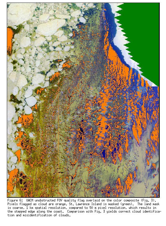
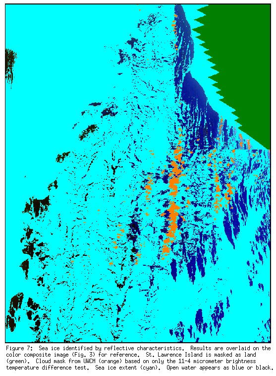
Using only the unobstructed FOV flag, clouds in the scene were masked. In this scene some areas of ocean were masked as clouds (Figure 6). Clouds were identified over areas of new ice or open water e.g., in the lower right quadrant, near the St. Lawrence Island coast, and in the left third of the scene (Figure 6). Cloud misidentification appeared to occur in the domain of daytime ocean (column one in Table 1), where the ice/snow background flag was set to off. Investigation of the individual cloud tests done in that processing path revealed that the most accurate mapping of clouds was obtained with a single cloud test, the 11 - 4 µ m brightness temperature difference test. When only this test was used as the cloud mask, clouds were mapped with high accuracy (Figure 7) as determined from visual analysis of the image.
The source of cloud misidentification is the visible reflectance cloud screening test. This is a single channel reflectance test for discriminating bright clouds over dark surfaces. The channel and reflectance threshold used in this test depend on the surface being viewed. In the daytime ocean domain (Table 1) this visible reflectance test used MAS channel 6 (0.66 µ m) with a reflectance threshold of 7.0%. Ocean pixels flagged as having no ice/snow background were misidentified as cloud by this test. No other cloud tests applied in this processing domain were found to misidentify cloud. The misidentification was caused by greater-than-expected reflectances from the ocean in MAS channel 6. The mean reflectance of the ocean under the misidentified clouds is 8.1%. Since this exceeds the reflectance threshold, these pixels were identified as cloud. Two possible reasons for the high ocean reflectances are: 1) the ocean surface was not totally ice-free, or 2) the sea surface was significantly wind-roughened. Plots of reflectance for features in the scene (Figure 5) indicate that some areas of the ocean had relatively high reflectance, assuming negligible atmospheric contribution to the signal. Also confounding the test was the fact that some of the new ice types had reflectances near those for cloud at visible wavelengths, but not in the infrared. The misidentification of cloud in this situation does not invalidate the use of the UWCM. Rather, it highlights the need for the user to be aware of and to make use of the individual cloud tests as necessary.
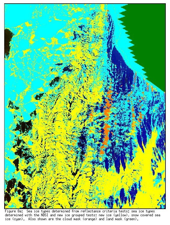
The ice by reflectance criteria group accurately (by visual interpretation) mapped the extent of sea ice, snow-covered and new sea ice in the scene (Figure 7). These selected reflectance criteria were based on sea ice reflectances reported in the literature and observed in the MAS data. Only sea ice extent was determined by this criteria group. With the many channels on the MAS and the MODIS sensors, it may also be possible to identify broad sea ice classes. Sea ice reflectance curves (Figure 5) suggest that two generalized classes, namely new sea ice and snow-covered sea ice, may be differentiated on the basis of reflectances. These classes are interpreted to be related to the World Meteorological Organization (WMO) stages of development, with new ice corresponding to stages that are < 10 cm thick and snow-covered ice corresponding to stages > 10 cm thick. New sea ice types exhibited reflectances intermediate between snow covered sea ice and water over the 0.5 - 0.9 µ m region (Figure 5). New sea ice reflectance characteristics could cause confusion with clouds in the scene (Figure 5), however the cloud mask removed this potential confusion. Another difference between snow-covered sea ice and new ice was noted in the 1.6 - 1.9 µ m region. In this spectral region, snow-covered sea ice has a local peak in reflectance (Figure 5) while new sea ice has a relatively uniform low reflectance (Figure 5).
These observed reflectance differences were used to create thematic maps of new, and snow-covered sea ice. Two methods of classifying ice were implemented. The intermediate reflectance of new ice over the 0.6 - 0.8 µ m region was approximately 60% lower than snow-covered ice and approximately 30% lower than young ice types (Figure 5). This intermediate reflectance (25% to 45%) was added as a criterion to the reflectance criteria group to identify new ice. A pixel meeting both the original criteria and this new ice criterion is identified as new sea ice. If it meets only the original criteria it is identified as snow-covered sea ice (Figure 8a).
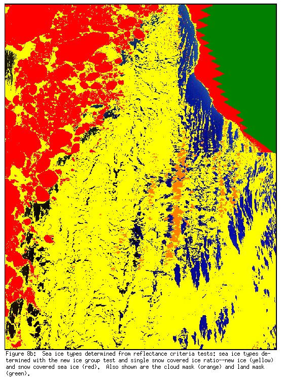
Also, snow-covered and new sea ice can be differentiated using the near-infrared ratio of MAS channel 12 (1.7 µ m) to channel 10 (1.6 µ m). Snow-covered sea ice has ratio values >= 1.1 and new ice has ratio values of < 1.1. This criterion test (snow-covered sea ice if ratio >= 1.1 and new ice if < 1.1), along with a threshold test in MAS channel 1 (0.55 µ m) can be used separate water from new ice and was implemented as a separate criterion group. This group resulted in a reasonably accurate map of snow-covered sea ice (Figure 8b).
Both maps of sea ice classes (Figure 8a and Figure 8b) agree with visual interpretation of ice type, and are in general agreement with general patterns of sea ice extent and type for the region as reported in previous studies (e.g. Massom and Comiso, 1994). Absence of in situ observations limit these results to qualitative discussion. However, they do show that additional information about sea ice beyond sea ice extent is possible with the MAS and MODIS sensors. For the MODIS sea ice algorithm only the criteria groups and tests given in Figure 4 will be used in the first version after launch.
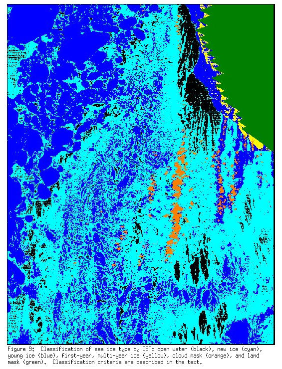
Sea ice extent (Figure 9) from the IST criteria group was in agreement with interpreted sea ice extent in Figure 3. The sea ice extent map created by flagging any pixel with an IST less than 271.4 K fails to make full use of the IST information. Ice classification is possible using IST because of the marked thermal contrast between open water, new ice and first-year and older sea ice types (Massom and Comiso, 1994). Also, the surface temperature of ice is strongly related, in principle, to ice thickness, allowing inference of ice thickness (Yu and Rothrock, 1996). Based on this information, a hypothetical three-classification sea ice map was created using the temperature ranges of the classes shown in Table 2. The ice-type map for this classification scheme is shown in Figure 9. New ice and young ice types are the dominant ice types identified. Some first-year ice was identified along the coast of St. Lawrence Island which is a mix of both fast ice and snow-covered land which was not masked by the land mask. Without surface observations this classification cannot be verified, but it is a reasonable classification for the region based on descriptions in Massom and Comiso (1994) for the area around St. Lawrence Island for the same time of year during 1988. The observed consistency of sea ice type and distribution as determined by the estimated IST method between the studies is encouraging.
Independent validation activities in support of the MODIS sea ice algorithm will be performed to determine the coefficients, modify the IST equation, and possibly to include dynamically-adaptive coefficients that can be adjusted for specific geographical regions, seasons, surface temperatures, or
a combination of parameters in order to increase accuracy of the IST.
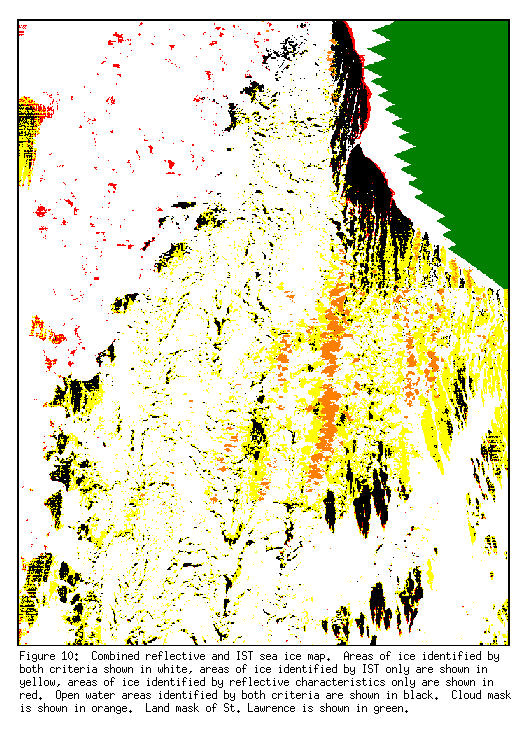
The motivation for combining the results of the two criteria groups is to enhance analysis and identification of sea ice, primarily in areas of new-ice formation when the reflectance characteristics of new sea ice make it difficult to detect and where the surface temperature is near the freezing point of sea water. Mapped sea ice extent was different in the reflectance and IST criteria groups. There are areas in the scene, (e.g. along the left third and right middle third of the scene), that appear to be open water in the color-composite image (Figure 3) that are not identified as ice by the reflectance criteria group for ice (Figure 7) but are identified as new ice by the IST (Figure 9) classification. Differences in sea ice extent between the two techniques are areas where there may be a mix of sea ice and open water or where other factors were affecting the surface characteristics. Horizontal striping in Figure 9 and Figure 10 suggest sensor performance effects in the thermal bands. The most certainty in the sea ice extent occurs where the two identification techniques (reflectance and IST (Figure 4)) agree (Figure 10).
Summary
Using reflectance and thermal data from MODIS or MAS it is possible to map sea ice extent and possibly classify sea ice type. The UWCM provided a reasonably accurate masking of clouds over sea ice when only specific cloud tests were considered in this analysis. Thus use of the cloud mask in polar regions may require an in-depth analysis of the cloud mask data content to maximize its effectiveness and accuracy. Albeit limited in scope, this work has been used to develop the MODIS sea ice algorithm. Algorithm development and analysis continues with MAS data, including comparison of results with SSM/I derived sea ice extent. It is anticipated that a similar capability for mapping sea ice will be obtained with the MODIS sea ice algorithm.
The MODIS sea ice algorithm is developed with the same criteria described here for mapping sea ice with MAS data (Figure 4) and is fully automated. Classification of sea ice type is not yet included in the MODIS algorithm. The algorithm will be bootstrapped with actual MODIS data using the coefficients reported here or with better determined coefficients from other studies with MAS. Initial estimated IST accuracies with MODIS data are anticipated to be poor and the coefficients adjusted frequently during the first year to improve accuracy. Validation studies are expected to be used to identify adjustments to the coefficients and to define sets of coefficients for use in specific regions (e.g. regions within the Arctic, or Antarctica) and possibly seasonal subsets for regions. Sea ice will be mapped both day and night with MODIS, though at night only the IST will be used. The MODIS cloud mask will be used for both day and night products. The UWCM does night time detection of clouds using thermal tests, however, performance of the cloud mask at night over sea ice is still being investigated and is expected to be lower than its performance during daytime.
The MODIS sea ice data product will be archived in Hierarchical Data Format-EOS (HDF-EOS) composed of scientific data sets and metadata. Sea ice derived from reflectance characteristics, estimated IST, sea ice extent by IST and combined sea ice extent (Figure 4) are archived as scientific data sets in the data product. Night time products will have only IST arrays. Extensive metadata (information about the data product) supporting EOSDIS Core System (ECS) services and containing quality assurance information and product summary information is also included with each product. Sea ice products are to be archived at the National Snow and Ice Data Center (NSIDC) in Boulder, Colorado (Scharfen et al., 1997). Sea ice products at 1 km spatial resolution are planned for swaths ("scenes") day and night of MODIS data. Gridded daily products at 1 km and 0.25° spatial resolution in Lambert azimuthal equal-area polar projection, and composite products of eight day and monthly at 0.25° spatial resolution are planned.
Acknowledgments
Thanks to N. Larsen (U. Alaska, Fairbanks) for thought-provoking discussions throughout the course of this project, and to A. Klein (Texas A &M University) for assistance with image production and review of the manuscript. Thanks to K. Strabala, R. Frey and L. Gumley for their important roles in coding the MAS cloud algorithm. Thanks also to anonymous reviewers for useful comments and suggestions that much improved the manuscript.
Relevant World Wide Web sites:References
Ackerman, S., Strabala, K., Menzel, P., Frey, R., Moeller, C., Gumley, L., Baum, B., Schaaf, C., Riggs, G., and Welch, R. (1996), Discriminating clear-sky from cloud with MODIS, Algorithm Theoretical Basis Document (MOD35), Version 3.0, 109 pp.
Allison, I., Brandt, R. E., and Warren, S. G. (1993), East Antarctica sea ice: albedo, thickness distribution, and snow cover. J. Geophys. Res. 98(C7):12,417-12,429.
Barnes, W. L., Pagano, T. S., and Salomonson, V. V. (1998), Prelaunch characteristics of the Moderate Resolution Imaging Spectroradiometer (MODIS) on EOS-AM 1. IEEE Trans. Geosci. Remote Sens. 36(4);1088-1100.
Carsey, F. D., Barry, R. G. and Weeks, W. F. (1992), Chapter 1. Introduction, In: Microwave Remote Sensing of Sea Ice (F. D. Carsey, Ed.), Geophysical Monograph 68, AGU, pp. 1-7.
Comiso, J. C. (1994), Surface temperatures in the polar regions from Nimbus 7 temperature humidity infrared radiometer. J. Geophys. Res. 99(C3):5,181-5,200.
De Abreu, R. A., Barber, D. G., Misurak, K., and LeDrew, E. F. (1995), Spectral albedo of snow-covered first-year and multiyear sea ice during spring melt. Ann. Glaciol. 21:337-342.
Grenfell, T. C., and Perovich, D. K. (1984), Spectral albedos of sea ice and incident solar irradiance in the Southern Beaufort Sea. J. Geophys. Res. 89(C3): 3,573-3,580.
Gumley, L. E., Hubanks, P. A., and Masuoka, E. J. (1994), MODIS Technical Report Series, Volume 3, MODIS Airborne Simulator Level 1B Data User's Guide, NASA Tech. Memo. 104594, Vol.3, 37 pp.
Hall, D. K., Riggs, G. A., and Salomonson, V. V. (1995), Development of methods for mapping global snow cover using Moderate Resolution Imaging Spectroradiometer data. Rem. Sens. Environ. 54:127-140.
Key, J. R., and Haefliger, M. (1992), Arctic ice surface temperature retrieval from AVHRR thermal channels. J. Geophys. Res. 97(D5): 5,885-5,893.
Key, J. R., Collins, J. B., Fowler, C., and Stone, R. S. (1997), High-latitude surface temperature estimates from thermal satellite data. Rem. Sens. Environ. 61:302-309.
King, M. D., Menzel, W. P., Grant, P. S., Myers, J. S., Arnold, G. T., Platnick, S. E., Gumley, L. E., Tsay, S., Moeller, C. C., Fitzgerald, M., Brown K. S., and Osterwisch, F. G. (1996), Airborne scanning spectrometer for remote sensing of cloud, aerosol, water vapor, and surface properties. J. Atmos. and Ocean. Technol. 13:777-794.
Lindsay, R., and Rothrock, D. (1993), The calculation of surface temperature and albedo of Arctic sea ice from AVHRR. Ann. Glaciol. 17:174-183.
Massom, R., and Comiso, J. C. (1994), The classification of Arctic Sea ice types and the determination of surface temperature using advanced very high resolution radiometer data. J. Geophys. Res. 99(C3):5201-5218.
McMillin, L. M., and Crosby, D. S. (1984), Theory and validation of the multiple window sea surface temperature technique. J. Geophys. Res. 89:3655-3661.
Minnett, P. J. (1990), The regional optimization of infrared measurements of sea surface temperature from space. J. Geophys. Res. 95:13497-13510
Parkinson, C. L., and Gloersen, P. (1993), Global sea ice coverage, In: Atlas of Satellite Observations Related to Global Change. (R. J. Gurney, J. L. Foster, and C. L. Parkinson, eds.) Cambridge University Press, pp. 371-384.
Perovich, D. K. (1990), The evolution of sea ice optical properties during fall freeze-up. SPIE Vol. 1302, Ocean Optics X. 520-531.
Perovich, D. K., Maykut, G. A., and Grenfell, T. C. (1986), Optical properties of ice and snow in the polar oceans. I: observations. SPIE Proceedings, Vol. 637, Ocean Optics VIII. 232-241.
Riggs, G. A., Hall, D. K., and Salomonson, V. V. (1996), Recent progress in development of the Moderate Resolution Imaging Spectroradiometer snow cover algorithm and product. In 1996 International GeoScience and Remote Sensing Symposium, Remote Sensing for a Sustainable Future, 27-31 May, 1996, Lincoln, NE. Vol 1:139-141.
Scharfen, G. R., Hall, D. K., and Riggs, G. A. (1997), MODIS snow and ice products from the NSIDC DAAC. SPIE Proceedings, Vol. 3117, In Earth Observing Systems II, (W.L. Barnes, ed.) 143-147.
Schlosser, E. (1988), Optical studies of Antarctic sea ice. Cold Regions Sci. Tech. 15:289-293.
United States Geological Survey. (1997), EROS Data Center Distributed Active Archive Center, http://edcwww.cr.usgs.gov/landdaac/1KM/land_sea_mask.html.
Washington, W. M., and Parkinson, C. L. (1986), An Introduction to Three-Dimensional Climate Modeling. University Science Books, Mill Valley, CA, 422 pp.
Yu, Y., and Rothrock, D. A. (1996), Thin ice thickness from satellite thermal imagery. J. Geophys. Res. 101:25,753-25,766.
Yu, Y., Rothrock, D. A., and Lindsay, R. W. (1995), Accuracy of sea ice temperature derived from the advanced very high resolution radiometer. J. Geophys. Res. 100(C3):4,525-4,532.
List of Tables
Table 1. UWCM domains and cloud screening tests used for the MAS scene. The spectral reflectance (R) and brightness temperature (BT) are listed. An × mark indicates that a test was done for that domain.
 <
<